Open Office How Can I Create a Formula to Show Numbers From One Sheet Onto Another?

Let's imagine a state of affairs where yous've got 2 columns in a Google spreadsheet: the 1st with prices, the 2nd with quantity of items, and yous need to multiply them in the tertiary column. What practise yous usually practice in this case? If you were similar me in the past, you'd compose a formula in the starting time row and copy-paste it in the other rows. A good quondam-school method that works fine.

But what if in that location are 1000 rows or even more? Annoying, right? Permit alone time consuming. Information technology can likewise cause a performance event since a bunch of like formulas slow down the whole spreadsheet. And, if you need to add a new value and create a separate row for it, Google Sheets volition non automatically copy the formula.

OK, so what's the solution here?

Actually, there is a dynamic and efficient way to address the discussed bug, and this manner is chosen ARRAYFORMULA.

What is ARRAYFORMULA?

In short, ARRAYFORMULA is a function that outputs a range of cells instead of only a single value and can exist used with not-assortment functions.

According to Google Sheets documentation, ARRAYFORMULA enables

"the display of values returned from an assortment formula into multiple rows and/or columns and the use of non-array functions with arrays".

Well, the definition kills any want to employ the function, but wait, do not jump to a conclusion. It is tremendously useful, and easier to utilise than it sounds like in the description.

To utilize it in Google Sheets, you tin either straight blazon "ARRAYFORMULA" or hit a Ctrl+Shift+Enter shortcut (Cmd + Shift + Enter on a Mac), while your cursor is in the formula bar to make a formula an array formula (Google Sheets will automatically add ARRAYFORMULA to the start of the formula).

Read more about Google Sheets shortcuts.

If you prefer watching than reading, check out this video tutorial by Railsware Product Academy about ARRAYFORMULA in Google Sheets

How does ARRAYFORMULA solve the problems?

• Since this is one single formula even for a huge dataset, you won't stop up with a lot of formulas, and your Google Sheets will run smoothly.
• ARRAYFORMULA is as well expandable – a modify in one place will expand down in the unabridged data range.
• And information technology is dynamic equally well. When a new row is introduced into the dataset, the formula will automatically be applied to information technology.

ARRAYFORMULA syntax

                =ARRAYFORMULA(array_formula)              

array_formula is a parameter that can be

• a range
• a mathematical expression using ranges of the same size, or
• a function that returns a result greater than one cell

ARRAYFORMULA example

Let'due south have a closer look at how the ARRAYFORMULA works. The easiest way to understand this is through an example.

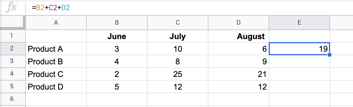
Allow'south say we have a dataset showing the quantity of four different products sold in the summer months

and we need to summate the total corporeality of sold products.

Sure, nosotros could do information technology past writing a formula in column Due east that adds B, C and D.

=B2+C2+D2

Or use the SUM part.

To find the sold quantity of B, C, and D products, you can copy the formula in E2 and and then paste information technology into the cells E3, E4 and E5

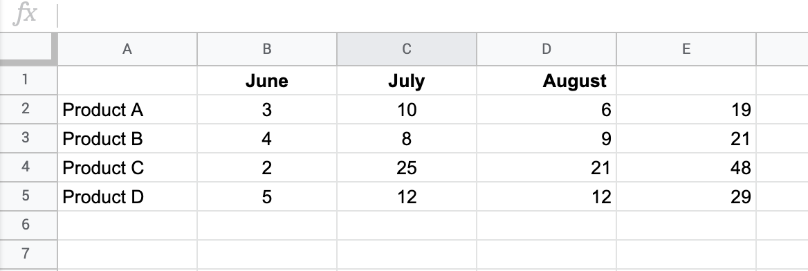
and then use SUM at the bottom of cavalcade E.

=sum(E2:E5)

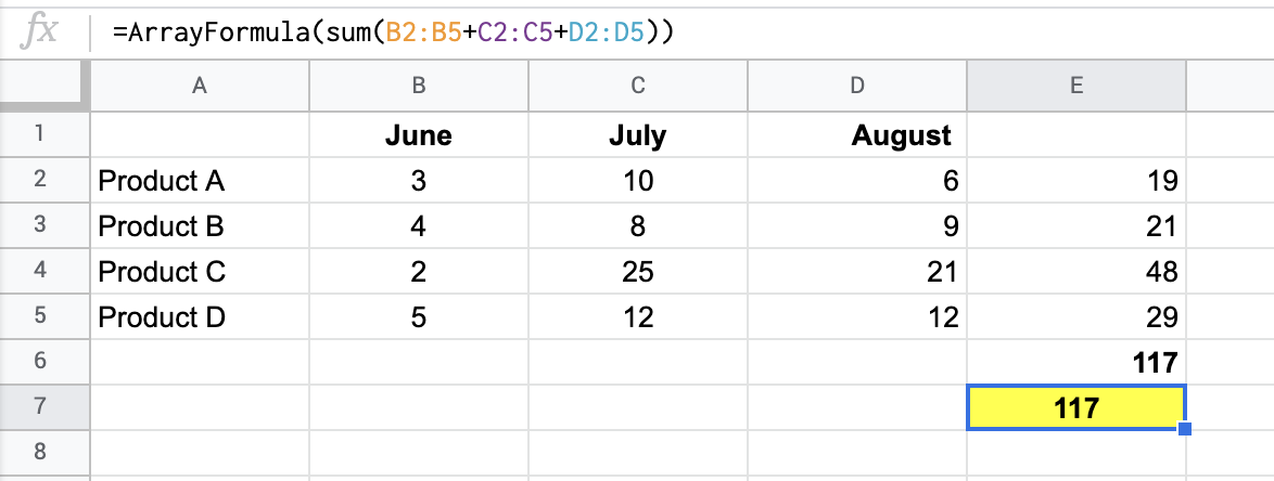
Nonetheless, the ARRAYFORMULA lets you skip all those steps and go directly to the answer with a single formula, which saves you time and energy if you've got 1000+ products.

In our case nosotros will have

=ArrayFormula(    sum(B2:B5+C2:C5+D2:D5) )

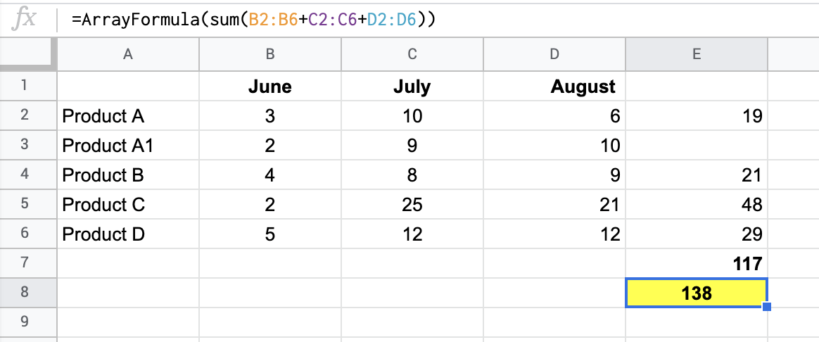
Now, I am adding a new range for Product A1.

ARRAYFORMULA takes into account the new range (changes B5 to B6, C5 to C6, D5 to D6 in the formula), and does the calculation, unlike SUM, which is expected for Google Sheets. Now the formula looks as follows:

=ArrayFormula(    sum(B2:B6+C2:C6+D2:D6) )

ARRAYFORMULA with IF function

As mentioned before, ARRAYFORMULA tin exist used with non-array functions. For example, with IF. To remind you, the IF function in Google Sheets works by performing a logical test that can just have ane of two outcomes: true or fake. Read more than about IF and other logical functions in Google Sheets,

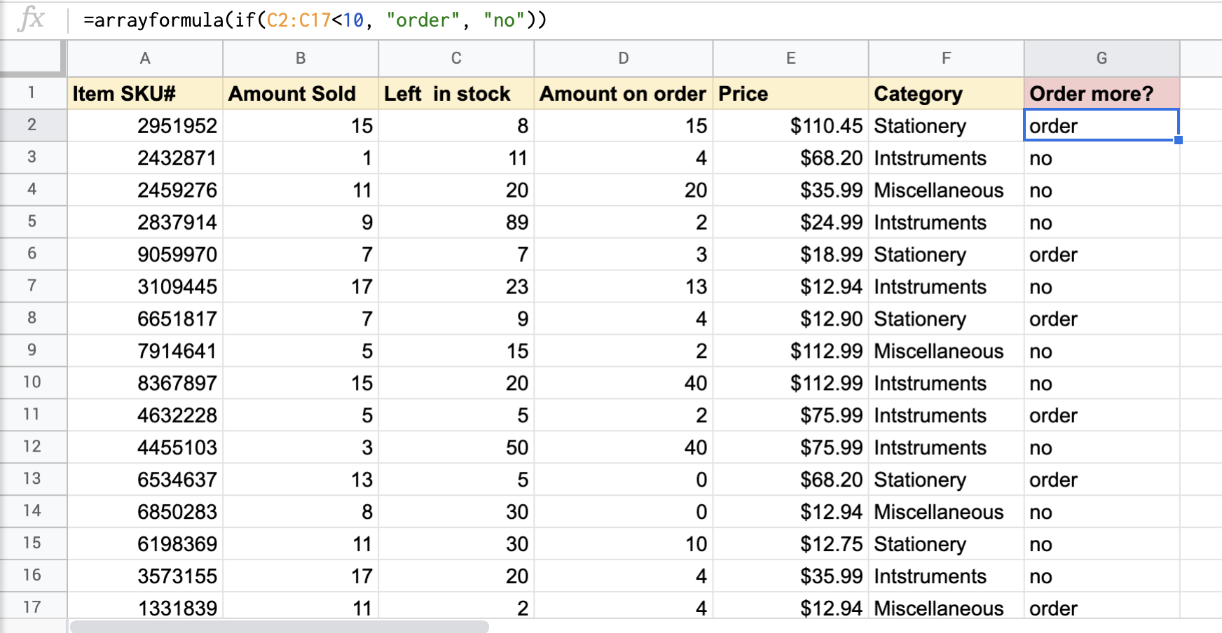
Permit'south encounter how to use the IF function and Assortment on the sales spreadsheet. Consider a standard IF statement that checks whether there are enough (more ten) items left in stock for next month.

In cell G2, I'd like to display the text "guild" if in that location are fewer than ten items left in stock, and "no" if the consequence is faux.

=if(C2<10, "order", "no")

The IF function does its calculation and, for this first detail, since there are only viii left in stock, the text "gild" is displayed.

Now let's run the test for each item, and this is where a single ARRAYFORMULA comes in handy. Type ARRAYFORMULA before IF, and it runs the IF statement across all the rows at one time. Cool, right?

=arrayformula(    if(C2:C17<10, "order", "no") )

SUMIF & SUMIFS with ARRAYFORMULA

Edifice on the previous example, allow's have a look at how ARRAYFORMULA can be used with SUMIF and SUMIFS Google Sheet functions.

SUMIF and SUMIFS are ii contained functions in Google Sheets. SUMIF is used for adding values based on one condition and the purpose of SUMIFS is to sum the values in a range, based on multiple conditions.

SUMIF + ARRAYFORMULA

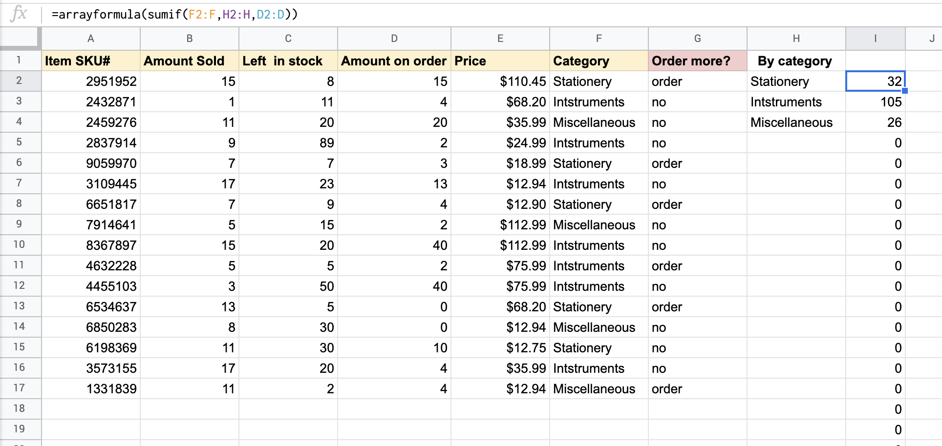
So, let's code an array formula for SUMIF. Let's say you demand to find out how many jotter items have been already ordered and you use SUMIF function, which returns you 32 in cell I2.

=sumif(F2:F,H2:H,D2:D)

And if you lot want to know the number of items already ordered for each category, the best way is to apply ARRAYFORMULA, which again will be extremely helpful if you have mode too many categories.

=arrayformula(    sumif(F2:F,H2:H,D2:D) )

SUMIFS + ARRAYFORMULA does non expand

With SUMIFS, things are a fiddling flake more complicated. Its syntax is:

                =SUMIFS(sum_range, range1, criteria1, [range2], [criteria2], ...)              

Unlike SUMIF, the SUMIFS does non expand the results even if you use ARRAYFORMULA with it. The logic is simple, since SUMIFS in Google Sheets returns the sum of an array conditionally, so it tin be nothing but a single result.

Let's check information technology out.

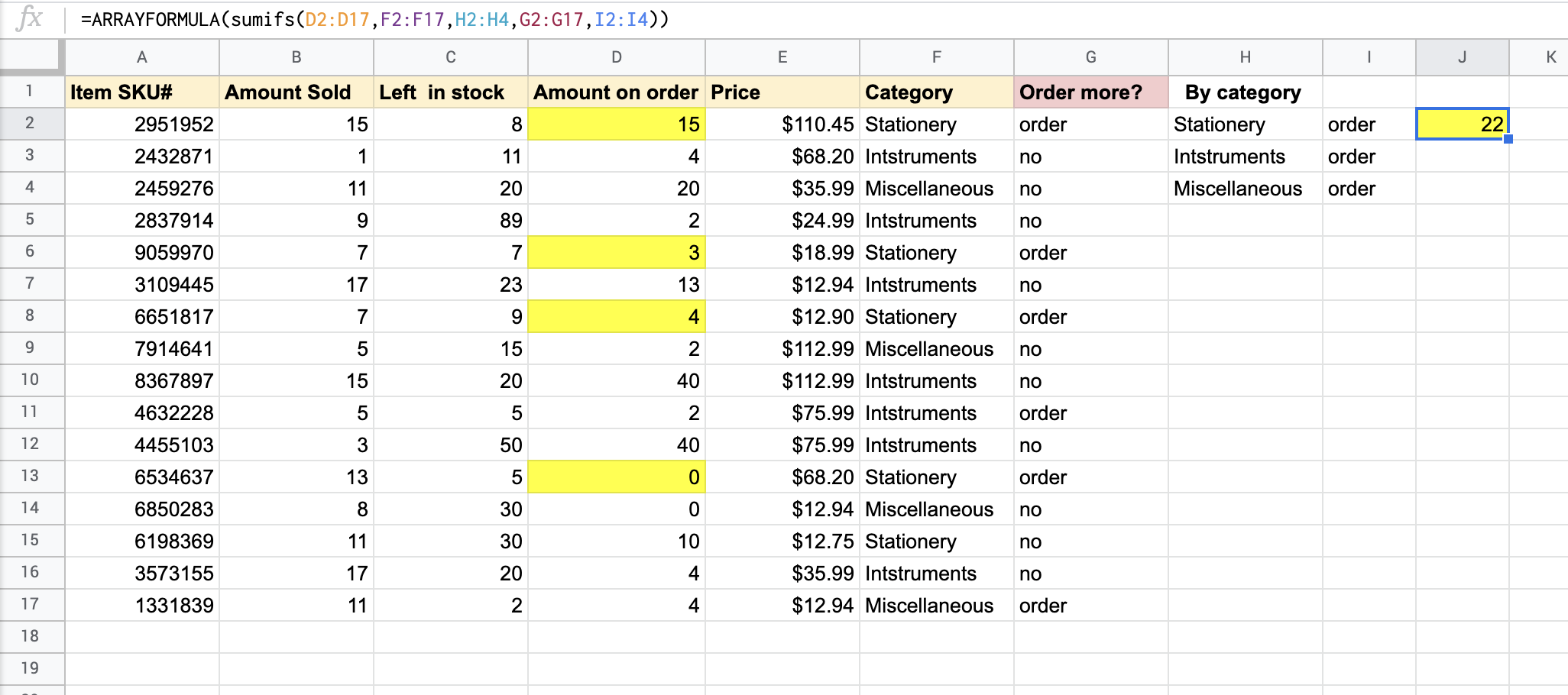
=sumifs(D2:D17,F2:F17,H2:H4,G2:G17,I2:I4)

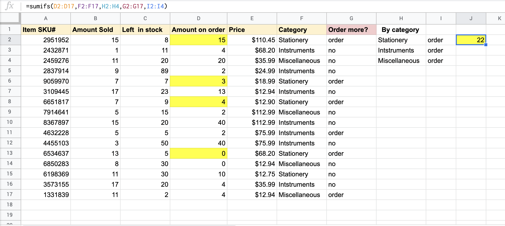
The SUMIFS in the above case sums the amount of "Stationery" items that needs to exist ordered. And, even if we nest SUMIFS with ARRAYFORMULA, information technology won't expand, but will return a single consequence one way or another.

=ArrayFormula(    sumifs(D2:D17,F2:F17,H2:H4,G2:G17,I2:I4) )

To solve this expanding issue, one should use alternative formulas. At that place are several options on how to address SUMIFS-ARRAYFORMULA-expansion problems, and the easiest i is with the assistance of SUMIF.

Alternative #1: ARRAYFORMULA and SUMIF

Actually, the SUMIF function can handle multiple criteria to expand the results, though in a slightly tricky way. The main tip here is to combine ranges and corresponding criteria using AMPERSAND (&).

=ArrayFormula(    sumif(F2:F17&G2:G17,H2:H4&I2:I4,D2:D17) )

And, as you lot tin can see, information technology is perfectly expandable.

Alternative #ii: ARRAYFORMULA, IF, LEN, VLOOKUP, QUERY

Another workaround is to use the combination of ARRAYFORMULA, IF, LEN, VLOOKUP, and QUERY functions. Looks complicated? Well, actually, it is. But the formula works perfectly, no doubt.

={"To order";   ARRAYFORMULA(IF(LEN(H2:H)=0,,     VLOOKUP(       H2:H&I2:I,        QUERY(         {F:F&M:Thousand,D:D},          "SELECT Col1, SUM(Col2) WHERE Col1 IS NOT Null Grouping BY Col1"       ),       two,       false     )   )) }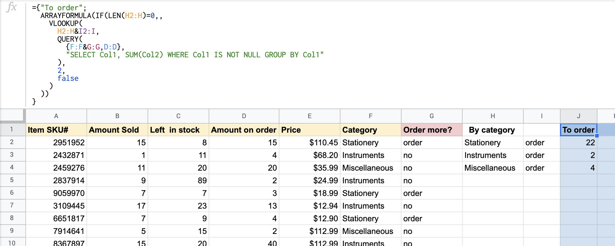

Can I use QUERY as an culling to SUMIFS+ARRAYFORMULA?

You may come upwards with the idea of trying to use something simpler, like QUERY solo, as some other internet resources advise. Well, nosotros tried to apply the following formula:

=query(A2:G,"Select sum(D) where F='"&H2&"'and Thou='"&I2&"' or F='"&H3&"'and Thou='"&I3&"' or F='"&H4&"'and 1000='"&I4&"' grouping past F,Grand characterization sum(D)''")

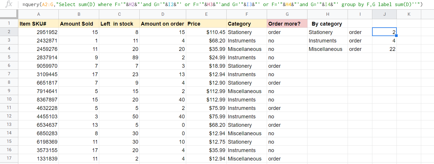
And logically it should have worked, but information technology hasn't as information technology returns results in random order, which is not convenient at all, to say the least. So, if you have no prejudices or limitations about using SUMIF, better cheque out the Alternative #1.

Read more nearly the ability of QUERY part in Google Sheets.

VLOOKUP and ARRAYFORMULA

For a lot of Google sheets users, mastering VLOOKUP is the turning point. That's when they are really getting comfortable with many functions and their application.

And, if you nonetheless haven't mastered information technology, open VLOOKUP by reading our dedicated post VLOOKUP Explained: How to Search Data Vertically in Spreadsheets.

As yous are probably aware, the principal limiting problem with VLOOKUP is that information technology only allows yous to look for a single value. However, the existent world often requires you to use ii or more criteria when looking up information from a database. To vertically look up multiple criteria, nest VLOOKUP with ARRAYFORMULA:

=ARRAYFORMULA(VLOOKUP({search-cardinal#1;search-cardinal#2;…}, range, column-index,[sorted/non-sorted])

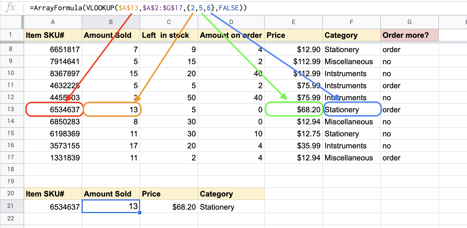
                =ARRAYFORMULA(VLOOKUP({search-central#1;search-fundamental#two;...}, range, column-index,[sorted/not-sorted])              

Let'due south have a look at the already-familiar table, assuming we want to search for Item SKU# and return Amount Sold, Cost and Category.

Since, we need VLOOKUP to render multiple columns, let's employ curly brackets "{}" to point the columns we want to return, and apply ARRAYFORMULA, so Google Sheets knows we're working with a range output, non a single value. My data table is in range A2:G17 and the search value is in A13, so the formula will exist every bit follows:

=ArrayFormula(    vlookup($A$thirteen,$A$2:$G$17,{2,five,6},FALSE) )

In fact, this is a regular VLOOKUP formula only, instead of a unmarried column, we use an assortment of columns in curly brackets: {2,5,vi}

VLOOKUP and ARRAYFORMULA in a real-life instance

Let's also consider another, more advanced case. For instance, let's see how Pipedrive users tin can import mixed data (some fields from one entity and some fields from some other) with the help of the ARRAYFORMULA-VLOOKUP combination.

Pipedrive, beingness an excellent tool itself, however doesn't offering enough options for reports customization and data flow configuration. And to be able to employ the reporting ability of spreadsheets and at the same time avoid manual copy-pasting, utilize Coupler.io which provides the Pipedrive Importer. Actually, with Coupler.io, you tin can import data not only from Pipedrive, merely from other popular apps, such as Jira, HubSpot, Airtable, and many more. Check out the bachelor Google Sheets integrations.

Pipedrive to Google Sheets importer, in particular, enables you to pull data separately from the post-obit entities: Deals, Persons, Organizations, Activities and Files.

Bank check out also the Pipedrive to Excel integration.

Though sometimes y'all may demand to extract data from different Pipedrive entities and combine information technology in a single sheet. In such a case, ARRAYFORMULA combined with VLOOKUP fits the beak.

Allow'due south encounter how it does the chore.

The first thing to do is to import fields:

• two fields from Persons (name, org_id.name, and org_id.accost)
• i field from Deals (formatted_value).

Stride 1: Set up two Pipedrive importers:

Parameters for the Pipedrive importer #1:

• Information entity: Persons
• Fields: name, org_id.name, org_id.address
• When configuring this importer, navigate to Destination => Testify advanced => type B1 into the "Cell address" field

This is how the imported Persons dataset looks:

Parameters for the Pipedrive importer #2:

• Information entity: Deals
• Fields: person_id.proper name, formatted_value

The field person_id.name is needed to vertically expect up the data.

This is how the imported Deals dataset looks:

Step 2: Apply the VLOOKUP formula nested with ARRAYFORMULA

One time yous've pulled the data, apply the post-obit VLOOKUP formula to the A1 cell in Pipedrive Persons sheet:

={"formatted_value";    iferror(       arrayformula(          vlookup(B2:B,'Pipedrive Deals'!A2:B,two,faux)       )    ) }

No dubiety, the ARRAYFORMULA-VLOOKUP combination, when used properly, is a tool that can save y'all tons of time and spare y'all a lot of busywork.

FILTER and ARRAYFORMULA

Another popular and useful function that proves beneficial when you lot need to discover data speedily is the FILTER function. It is used to conditionally filter the specified data range to get the required info. This Google Sheets function has already been explained in the FILTER How-To Guide, simply permit's reconsider the awarding of FILTER with ARRAYFORMULA.

In the sales spreadsheet, let's filter out duplicates – in our case, the identical sales numbers. Since there is no direct office in Google Sheets to cope with the task, the optimal workaround will be to utilize FILTER with UNIQUE, ARRAYFORMULA, and COUNTIF:

=filter(    unique(C2:C),    arrayformula(       countif(C2:C,unique(C2:C))>1    ) )

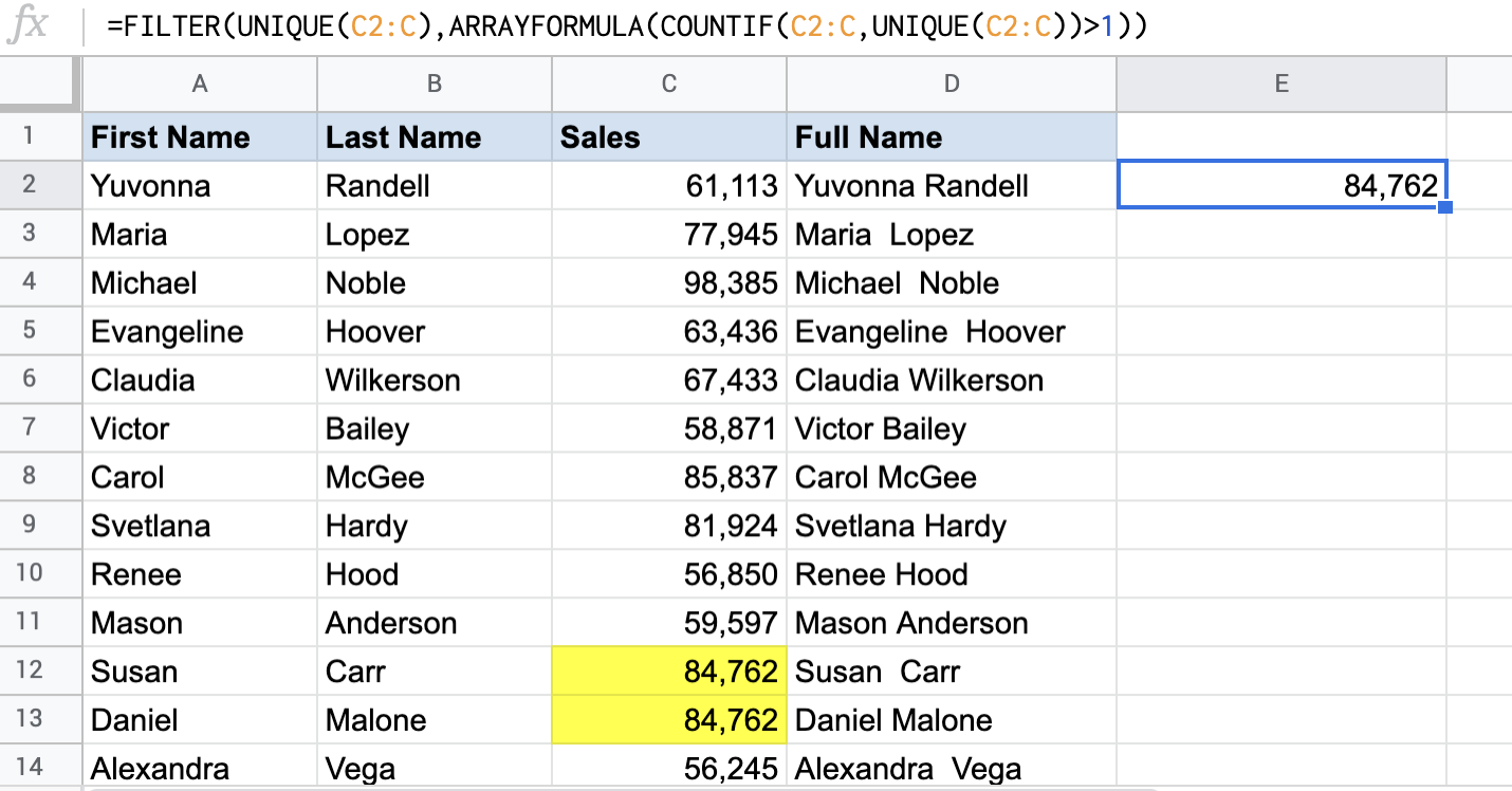
As you lot can see, the formula meets the challenges and returns ane duplicate.

How to employ ARRAYFORMULA to combine columns in Google Sheets

ARRAYFORMULA also helps y'all do manipulation with a text. You lot tin really combine a text with a text, a text with a number, and a text with a engagement in Google Sheets and utilise ARRAYFORMULA to that combination.

For case, if nosotros accept a list of, permit'south say, sales managers, and need to combine the first and last names. To get the proper name and the surname of the start sales manager, employ the post-obit formula:

=A2 &" "& B2

The full proper noun appears in a single cell, E2. Read more about Merging Data in Google Sheets.

So, permit'southward use the ARRAYFORMULA function to have all the names and surnames coupled.

=arrayformula(A2:A14 &" "& B2:B14)

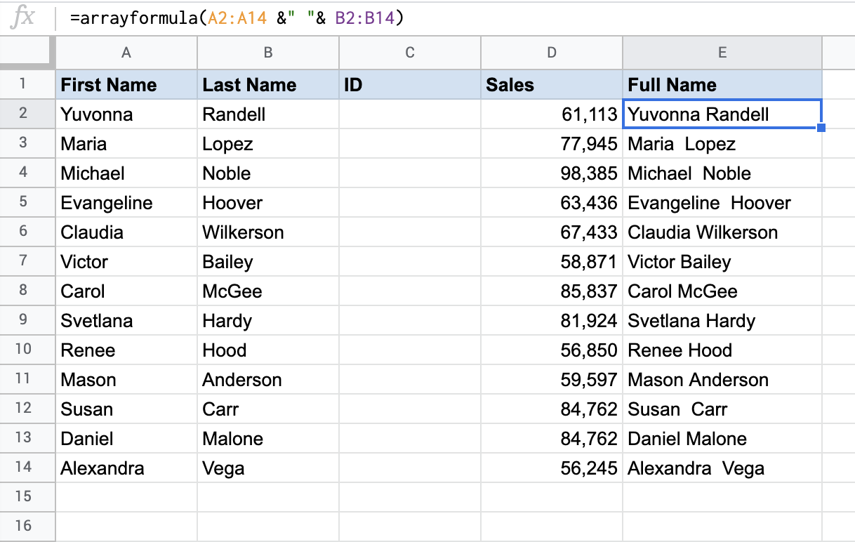
Applied but in E2, the formula automatically expanded to the other cells below.

Bare cells challenge in ARRAYFORMULA output

When you lot work with the ARRAYFORMULA function, yous have to exist careful with the array sizes. They should always exist the same, for example, F2:F17&G2:G17. Otherwise Google Sheets won't carry out the adding. As an option, not to sweat as well much, you may use the infinite range, as we did with SUMIF.

=arrayformula(    sumif(F2:F,H2:H,D2:D) )              

But, in this example, yous may face another challenge – extra blank cells in your formula output. In my instance with ARRAYFORMULA+SUMIF in I2, if there is the limited range H2:H4, all will work well.

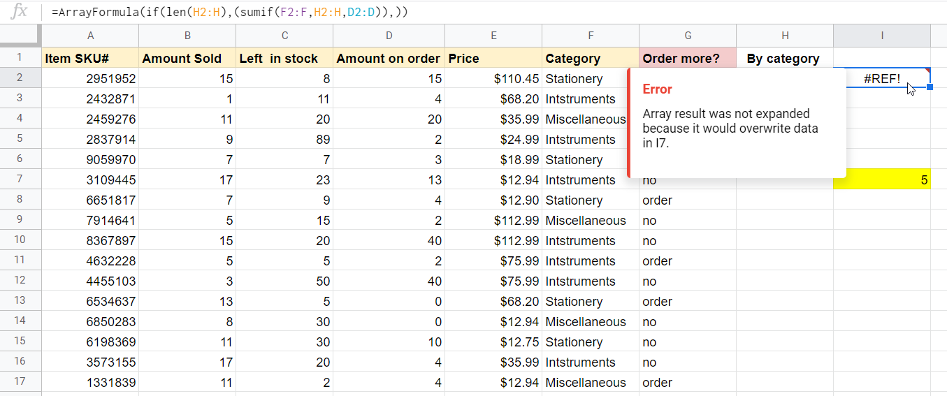
Though, if you lot change it to H2:H, SUMIF will treat this range as the one containing the criteria and will sum the column accordingly.

Well, it may spoil the looks, let alone litter upward the whole spreadsheet, simply, most chiefly, when you enter any value in any of those cells, the formula will return a #REF! Error.

And this happens non just with SUMIF, but with other formulas equally well. Then, let'south see how to remove them.

So, to remove extra bare cells returned by ARRAYFORMULA nested with SUMIF in Google Sheets, we can use the FILTER function to filter out blank cells in the criteria that cause the extra zeros and the blank cells correspondingly.

=ArrayFormula(    sumif(F2:F,filter(H2:H,H2:H<>""),D2:D) )

Or, alternatively, you lot can use IF+LEN and information technology volition do the same task.

=ArrayFormula(    if(len(H2:H),(sumif(F2:F,H2:H,D2:D)),) )

But, different the option with FILTER, IF+LEN won't help to avoid the issue with #REF! Error and volition likewise return it if you enter whatsoever value in blank cells, so be careful!

That's the curtain?

Inappreciably. The Google Sheet ARRAYFORMULA function is a really multi-purpose tool and can be used with many other combinations and applications not covered here. If you accept whatsoever in mind and want to hash out them, comment below and nosotros'll elaborate.

Equally for now, skillful luck with you data, and every bit Ben Collins, Google Sheets developer and data analytics teacher, wrote in his blog, "Hip, Hip Array!"

Dorsum to Blog

Access your data

in a simple format for free!

Start Free

vazquezfriest.blogspot.com

Source: https://blog.coupler.io/arrayformula-google-sheets/

Share this post